Today we will see how you can add a drop-down list in a Microsoft Excel cell. That is, a cell in which you can choose which value you want from a list. This is a very useful feature for spreadsheets and plantillas where the same options are always repeated.
It is a quick and easy way to give a professional touch to an Excel sheet and also make life easier for those who have to fill it in. We will see how to do it so that the data is based on a fixed list and also on the content of other cells. Excel files can be opened in other apps, remember, but if you use another one the way to proceed might be different.
Select cell
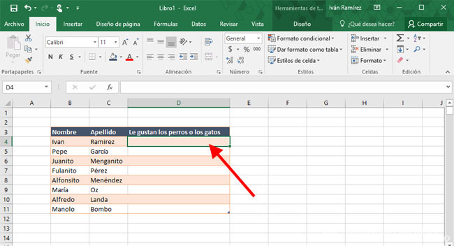
Let’s assume that you already have a half-done excel sheet and you just want one of the cells to become a drop-down list. The first step is to select the cell that you want to be a list. If there are several, don’t worry, select one first and then you can copy the same style to all the others.
Go to the Data tab
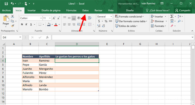
Actually creating a list of options in Excel is very simple, but what is more difficult is to find the option. First of all, click on the Data tab to open it, because the option we are looking for is found here.
Click on ‘Data validation
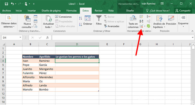
Now click on the Data Validation button, which is usually found in the Data Tools group. In some versions of Excel it is a rather small button, where you can barely make out the icon (which is two cells, one with an Ok symbol and one of the opposite).
Choose ‘List
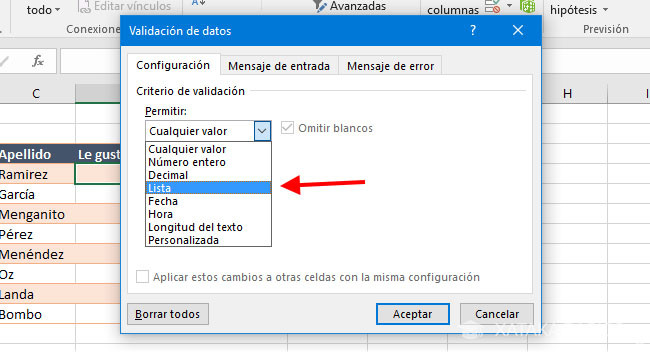
In the first drop-down list, the one under the heading Allow, choose the List option. The other options allow you to limit the contents of the cell to different formats such as numbers, dates, times and so on.
Adds items to the list
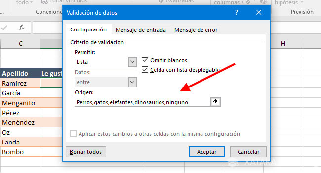
Next you have two options: either you type the items you want to be available in the list, or you select a range of cells that contain them. The first one is easier, as you only have to type the items you want to be in the list separated by a comma. For example, Banana, Mango, Pear, Apple.
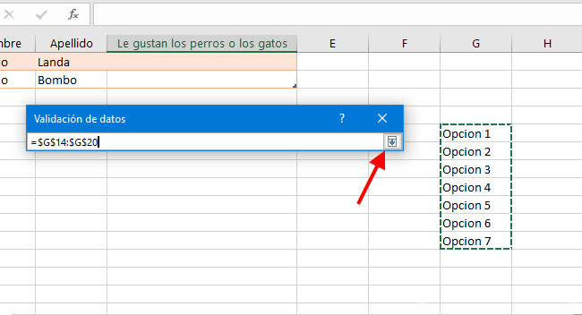
If you want the list options to be based on other cells, click on the arrow icon to minimize the Data Validation window, which will then be floating, and select the cells containing the data. When you are done, press Enter on the keyboard or press the arrow button again.
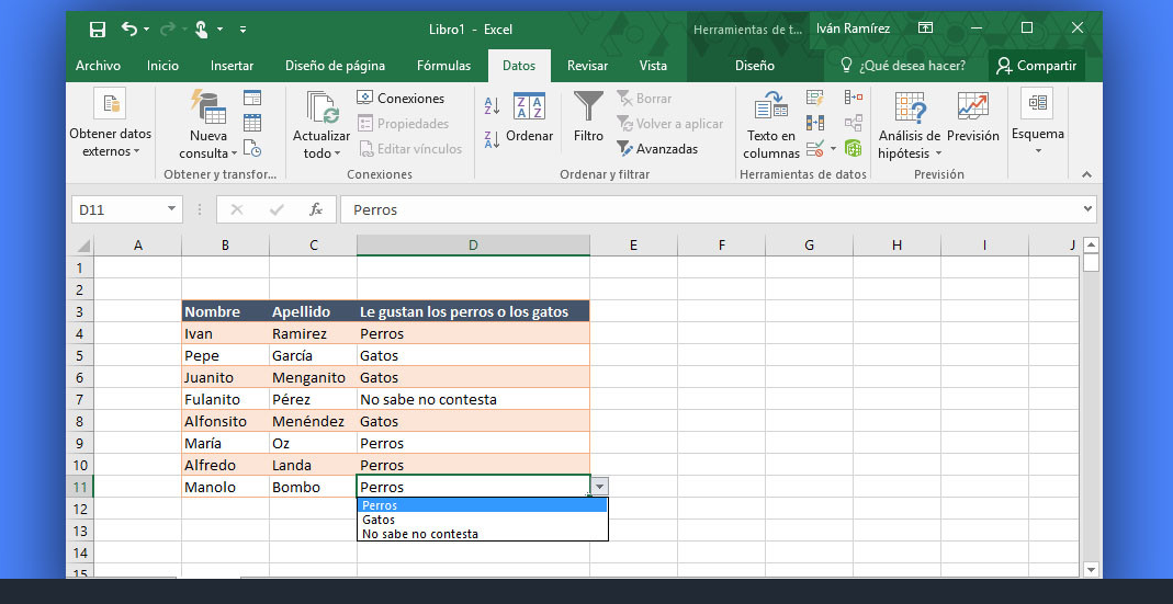
That’s it, now copy the cell (if you want)
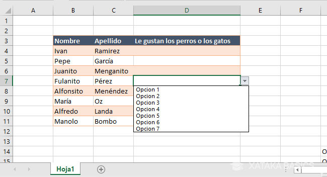
From this moment on, when you click on that cell, the button to display the options will be shown, which you can choose directly from the list. If you want to use this same validation (i.e. the same list) in other cells, instead of repeating the whole process, the easiest way is to copy it to the Clipboard and paste it in the rest of the cells where you want it to appear as well.