Today we are going to explain how to lock columns, rows and cells in Excel, in all the possible meanings that this can have. We will discuss all possible locks, from locking rows and columns to splitting the screen and, of course, protecting some cells from being editable.
First we will tell you how to freeze rows and columns, so that they remain fixed as you scroll through the spreadsheet. Then we will see how to split a spreadsheet, with a similar result. Finally, we will explain how to protect a spreadsheet so that some of its cells cannot be edited. Excel files can be opened in other apps, remember that, but if you use another one the way to proceed might be different.
How to immobilize (fix) rows and columns
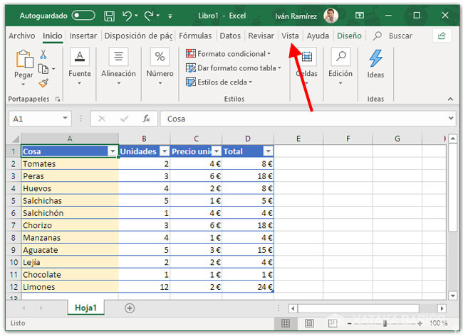
If you came to this article looking for how to make some Excel columns or rows stay fixed when using scrolling, this is what Excel calls pinning. Whether you want to freeze rows or columns, you should go to the View section of the tools.
Then click on Freeze, which displays three possible options: freeze panels, freeze top row and freeze first column. The result is similar, as we will see below.
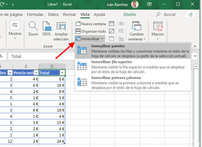
- Freeze panes: creates a split based on the currently selected cell. Use this option if you want to freeze both rows and columns, or if the row (or column) you want to freeze is not the first one.
- Freeze top row: Leave the first row of the spreadsheet static while scrolling vertically, leaving it always visible.
- Freeze first column: Leave the first column of the spreadsheet static while using horizontal scrolling, being always visible.
Immobilize top row
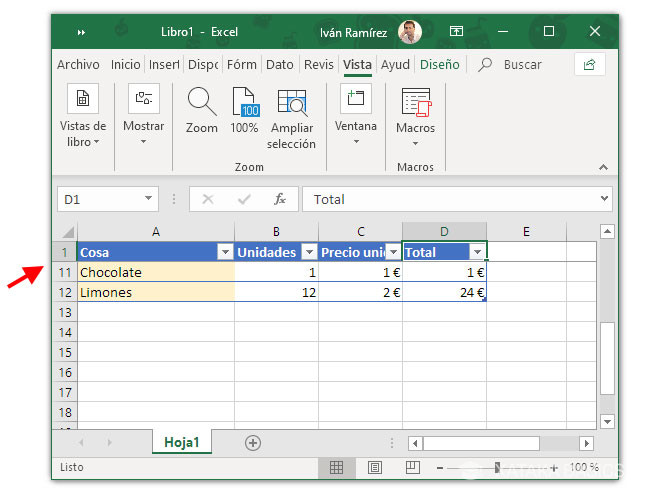
If you chose to freeze the top row, the result is something similar to the previous image. Note that when scrolling, the first row remains visible. In the above example, this allows us to follow what each item in the list is, something that would be impossible in a very long list.
Immobilize first column
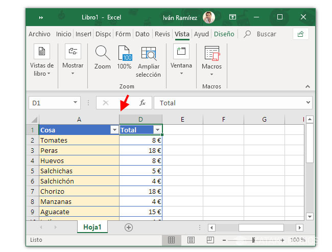
If you chose to freeze the first column, the result is the same, but applied to the column. That is, the first column remains always visible when you use the spreadsheet scrolling. In the above example, it allows us to see what each item is, something that would be more complicated in tables with a lot of data.
Immobilize panels
The most complex option is to lock panels. It is basically a combination of the two previous ones, since it locks both rows and columns. It does this based on the cell you have selected at that moment, which will act as a kind of axis for this immobilization. It is similar to the Split option that we will see next, although it is not quite the same.
Divide
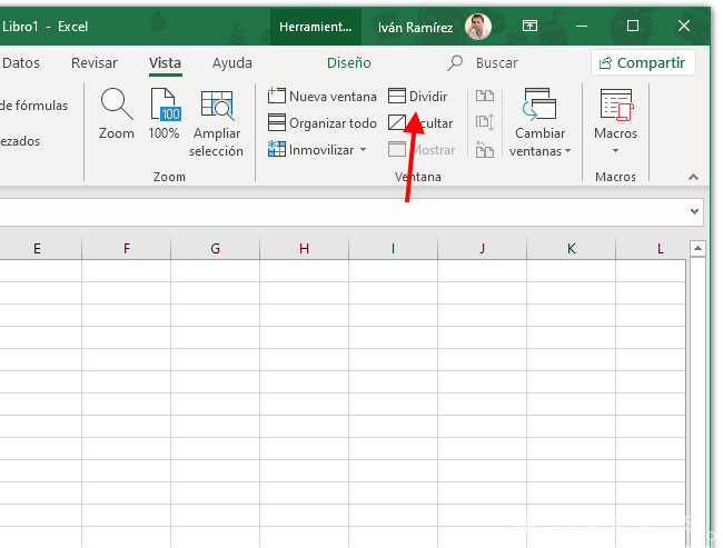
Pinning panels and splitting are almost the same thing, though not quite. Basically it is like splitting the screen into several views showing the same spreadsheet, so that you can control the scrolling separately in each area and thus see different parts of the same spreadsheet at the same time. To use this option you must go to the View section and click on Split.
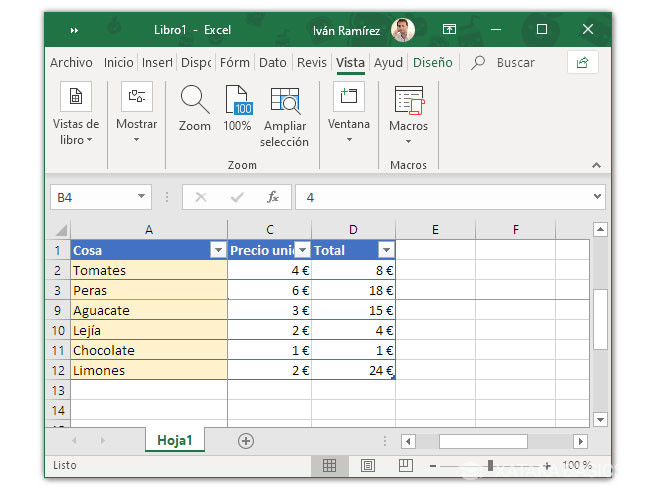
When you do this, a border appears in the middle of the spreadsheet that divides the area into four parts. You can scroll separately in each part to show different parts of the spreadsheet.
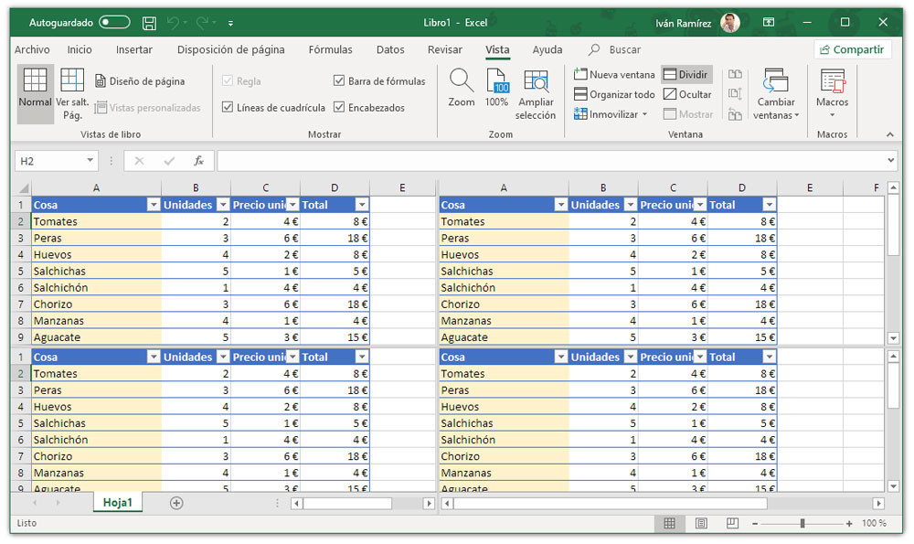
It is a similar option to pinning panels, although the difference goes beyond the fact that in this case a thick border is displayed. In addition, each area can show any part of the spreadsheet, which is not the case with pinned. In this way, it is possible to see the same rows in the different divisions, something that is impossible using locking.
How to lock cells so that they cannot be edited
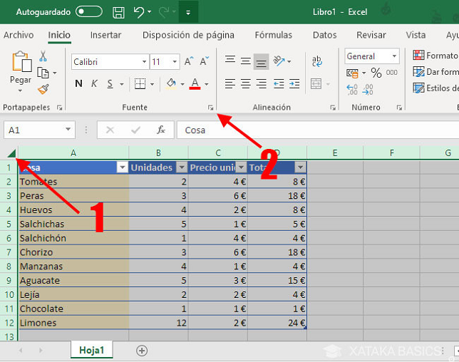
If you are looking to prevent certain rows, columns or cells from being editable, in that case you should know that the process needs a few intermediate steps. First of all, you need to select all the rows of the sheet (you can use the button in the corner (1)) and then click on the Source button (2), inside Home.
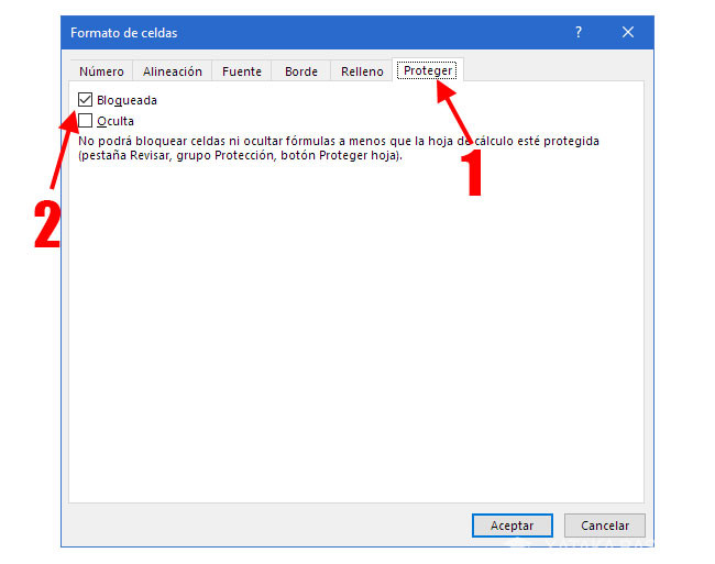
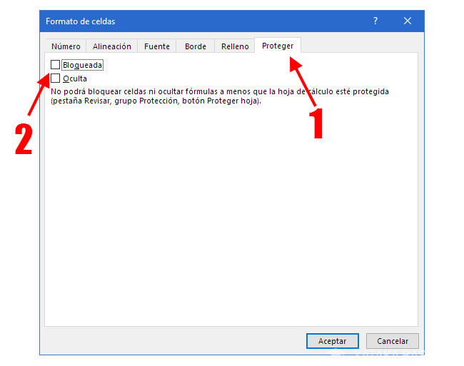
Go to the Protect section and uncheck the Locked option. That is, what we will do is to unlock all the rows, because our interest is that only a few cells are locked. This setting does not apply yet, because the sheet is not protected.
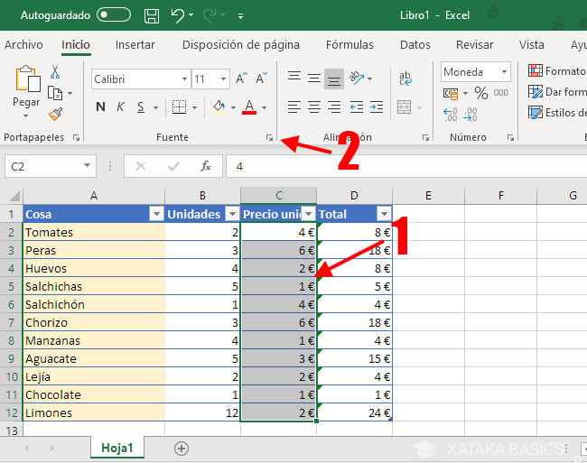
Next you must select the rows you want to protect and repeat the previous process. That is to say, keeping the previous selection, enter the Excel Home section and click on the Source button (2).
Now you must go to the Protect tab (1) and check the Locked box. This means that this cell (or the selection you had) cannot be edited unless the sheet is unprotected. As before, the change is not yet applied, as the sheet will be unprotected.
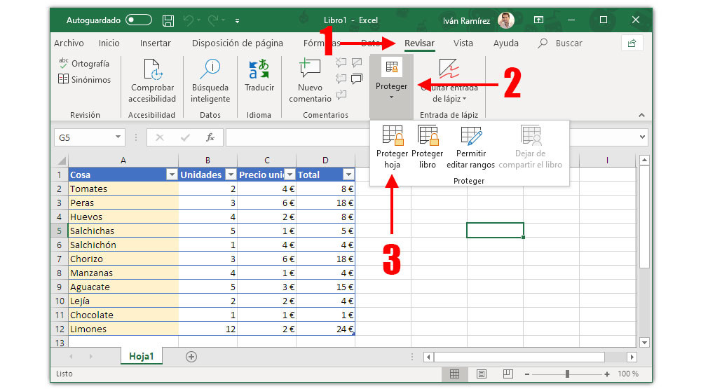
For the above steps to take effect you must protect the sheet. You do this by going to the Review tab (1) and clicking on Protect (2), then choose Protect sheet (3). If you want to protect the whole file and not just the current sheet, click Protect workbook instead.
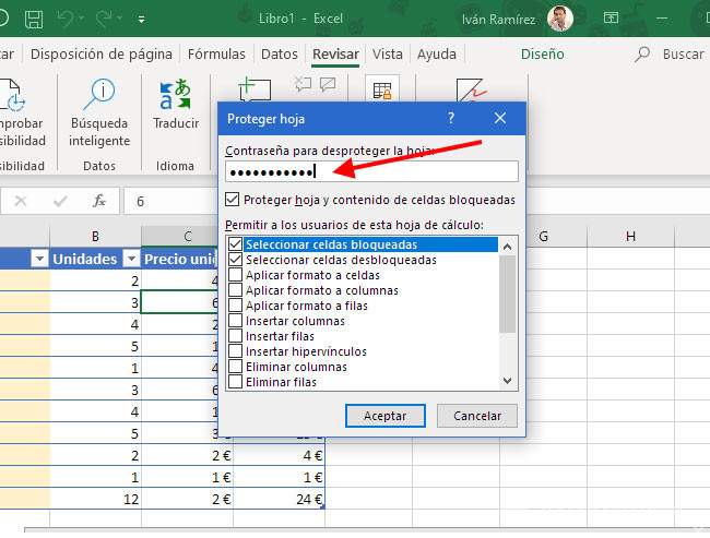
Now it is time to choose a password to protect the Excel sheet. You can type in any password you like, but make a note of it because you will need it to make changes later. Excel prompts you to type the password again before continuing. You do not need to touch anything in the options.
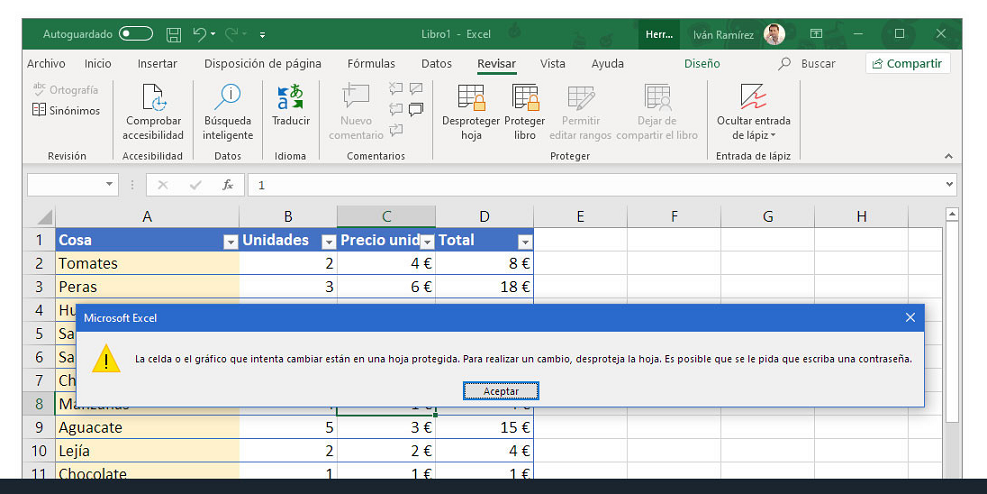
That said, the Excel sheet will be protected, but since we manually unlocked all its cells, only those we manually selected will be protected. In this case, when someone tries to edit a forbidden cell, Excel displays the message “The cell or chart you are trying to change is on a protected sheet. To make a change, unprotect the sheet. You may be prompted to enter a password”.
Indeed, if you ever need to edit some of these cells, you will first need to unprotect the sheet (following the same steps we used to protect it). You will need to provide the same password you used.