Excel is an excellent tool for storing and managing data. Subsequently, the data can be used to perform tasks such as data analysis or accounting. But sometimes duplication of data can occur. And duplicate values in Excel can make the aforementioned tasks more difficult.
Duplication of data can occur in a spreadsheet when records from multiple sources are combined. It can also occur when a particular piece of data is accidentally entered twice. In this article, we will look at some simple ways to remove duplicate values in Excel. When a duplicate value is deleted, it does not affect any other values outside of its cell or table. However, since the deletion of these values is permanent, it is advisable to double check before deleting them.
First we will see how you can filter by single value in Excel. Then, we will see how you can remove duplicate values. Finally, we will look at some formatting techniques. So, without further ado, let’s start with the first method for removing duplicate values in Excel:
Method 1: to filter single values in Excel
Filtering unique values is a task quite similar to removing duplicate values. Both tasks help to present a list of unique values in the spreadsheet. There is, however, one major difference. Filtering data will only temporarily hide duplicate values. Removing duplicate values will remove them permanently. Therefore, it is always advisable to filter first and check for unique values before removing duplicates.
To filter by unique values, follow these steps:
- Open Excel and click on the Data tab.
- In the Sort Filter group of the Data tab, click Advanced.

- You must enter the range of cells or the table you want to check in the pop-up window.
- In case you want to filter the values instead, click Filter list instead. To copy the filter results to another location (recommended), click Copy to another location. Add a cell reference in the Copy to box below.

- Checkmark “Single records only” and then click OK.
The unique values for the range will be copied to a new location.
Method 2: to remove duplicate values in Excel
A value can be said to be a duplicate value if all the values in one row are identical to all the values in another row. It is worth noting that when Excel looks for duplicate values, it only checks what appears as raw data in the cells. It cannot discern the meaning or values of this data, so there may still be some duplicate values left in the spreadsheet. For example, two values 01/15/2019 and January 15, 2019 in two different cells will not be identified as duplicate values since the date format is different in the two cases.
To remove duplicate values in Excel, follow these steps:
- In Excel, select the range of cells you want to check. Or make sure the active cell is in a table.
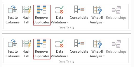
- Now click on the Data tab.
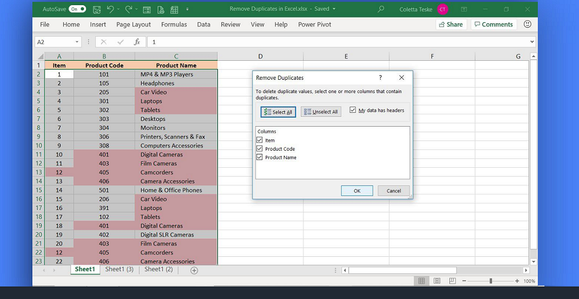
- In the Data Tools group of the Data tab, click Remove duplicates.
- Now, in the new pop-up window, select one or more columns. To select all columns, click Select all. To deselect all columns, click Deselect all. Or if you want to select particular columns, simply check the columns you want to check.
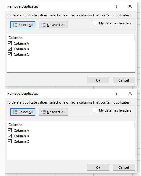
Note: this operation will remove data from all columns. The value of the columns you select will be used as a key to search for duplicates in all other columns. In case a duplicate is found in these columns, the entire row will be deleted, even from other columns in the range.
- Click OK. A message will appear. It will indicate the number of duplicate values that were deleted or the number of unique values remaining. Click OK.
Note: To undo any changes, simply press Control + Z.
Method 3: Formatting techniques for filtering unique values in Excel
We will discuss two different types of formatting techniques, quick formatting and advanced formatting.
Fast formatting:
- In Excel, select at least one cell within a range or table.
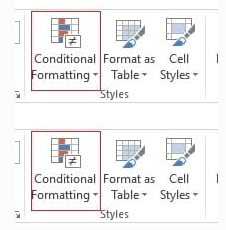
- Now click on the Home tab.
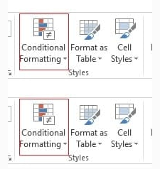
- In the Style group of the Home tab, click the small arrow for Conditional Formatting to expand it.
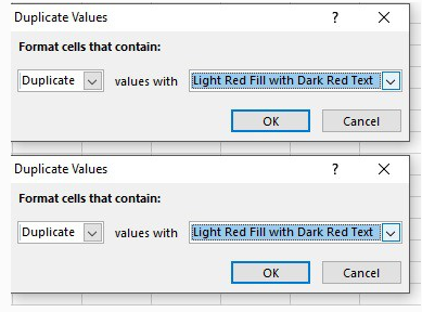
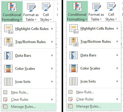
- Select Highlight cell rules and then Duplicate values.
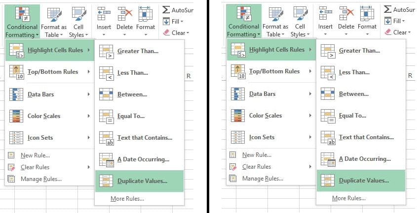
- Enter a specific format and select Duplicate or Single. Then click OK.
Advanced formatting:
- In Excel, select at least one cell within a range or table.
- Now click on the Home tab.
- In the Style group of the Home tab, click the small arrow for Conditional Formatting to expand it.
- Select Manage rules. A Conditional Formatting Rules Manager window will appear.
- What would you like to do next?
- If you want to add conditional formatting, select New rule. The New formatting rule window will appear.
- If you want to change a conditional format, first verify that you have chosen the appropriate worksheet or table in the Show formatting rules for list. (If you want to choose a different range of cells, click the collapse button to minimize the active window. You can then select an additional range of cells and expand the minimized Applies to window again). Now, simply select the ruler and click Edit ruler. The Edit formatting ruler window will appear.
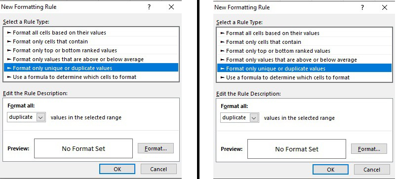
- Click Format only single duplicate values under the Select a rule type tab.
- In the Edit rule description window, choose Single or Duplicate in the Format all list. Click on Format. The Format Cells window will appear.
- Select all the things (font, number, fill formatting, border) you want to apply when the specified condition is met with a particular cell value. Now click OK.
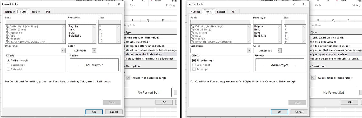
Note: You can select several formats. All formats you have selected are displayed in the Preview pane.
Hopefully, these methods will serve your purpose. If you need more help, you can consult the online MS Excel Answers community. Or if you need specific assistance, you can ask for help in the Excel technology community.